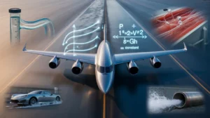
From the graceful curve of an airplane wing to the precise operation of a medical nebulizer, the invisible trade-off between fluid speed and pressure governs countless phenomena. Bernoulli’s equation quantifies this exchange, showing how static pressure, dynamic pressure, and gravitational potential energy redistribute along a streamline while their total remains conserved in ideal flow. It stands as one of fluid mechanics’ most powerful bridges between classical Newtonian mechanics and practical engineering.
Bernoulli’s Equation
P + ½ρv² + ρgh = constant (along a streamline)
- P: static pressure (Pa) — force per unit area exerted by the fluid
- ρ: fluid density (kg/m³)
- v: flow velocity (m/s)
- g: gravitational acceleration (9.81 m/s²)
- h: elevation above reference (m)
½ρv² represents dynamic pressure; the entire left side is mechanical energy per unit volume.
What Bernoulli’s Equation Truly Reveals
Bernoulli’s principle states that in steady, ideal fluid flow, an increase in velocity corresponds to a decrease in static pressure (or potential energy). This is energy conservation in motion: faster bulk flow means molecules carry more ordered kinetic energy, reducing the random collisions that manifest as pressure on surfaces. It explains lift, flow metering, and everyday pressure-velocity relationships without invoking “suction.”
Historical Foundations and Daniel Bernoulli’s Insight
Published in 1738 in Hydrodynamica, the equation emerged from Daniel Bernoulli’s studies of fluid pressure and motion, influenced by his father Johann and contemporaries like Leonhard Euler. Bernoulli applied the work-energy theorem to fluids, treating them as systems of particles. This work laid groundwork for Euler’s equations of inviscid flow and modern potential flow theory.
The Full Bernoulli Equation: Term-by-Term Analysis
Static pressure (P): The thermodynamic pressure measured perpendicular to flow, as in a wall tap.
Dynamic pressure (½ρv²): Kinetic energy density of the directed motion.
Hydrostatic term (ρgh): Gravitational potential energy per unit volume.
In horizontal flow, the equation simplifies to P + ½ρv² = constant, highlighting the classic pressure-velocity inverse relationship. Units confirm consistency: all terms have dimensions of pressure (N/m² or Pascals).
Step-by-Step Derivation from First Principles
Consider steady flow of an incompressible, inviscid fluid along a streamline. Take a small fluid element of volume dV and mass dm = ρ dV.
- Pressure work: Net work done = (P₁ − P₂) dV
- Kinetic energy change: ½ dm (v₂² − v₁²)
- Potential energy change: dm g (h₂ − h₁)
Conservation of mechanical energy (no viscous losses, no heat transfer):
(P₁ − P₂) dV = ½ρ dV (v₂² − v₁²) + ρ g dV (h₂ − h₁)
Dividing by dV yields the Bernoulli relation. This derives rigorously from integrating Euler’s equation along a streamline for irrotational flow.
The Continuity Equation: Essential Companion
For incompressible flow, the continuity equation A₁v₁ = A₂v₂ (or ρAv = constant for compressible) enforces mass conservation. A constriction increases velocity, which—via Bernoulli—decreases static pressure. This pairing underpins the Venturi effect and most practical calculations.
Worked Examples: From Basic to Advanced
Example 1: Horizontal Pipe (Beginner)
Water flows at 1.5 m/s in a 6 cm pipe, narrowing to 3 cm. Calculate pressure drop (Δh = 0, ρ = 1000 kg/m³).
Continuity: v₂ = 1.5 × (6/3)² = 6 m/s
P₁ − P₂ = ½×1000×(36 − 2.25) = 16.875 kPa
Example 2: Torricelli’s Theorem (Classic)
Speed of efflux from a hole at depth h: v = √(2gh). This follows directly when P₁ = P₂ (atmospheric) and v₁ ≈ 0.
Example 3: Airplane Wing Lift (Intermediate)
Air (ρ ≈ 1.225 kg/m³) travels at 65 m/s below and 80 m/s above a wing section. Approximate ΔP ≈ ½ρ(v_upper² − v_lower²) ≈ 1.4 kPa. Integrated over area and combined with circulation theory, this contributes significantly to lift.
Example 4: Advanced Venturi Meter with Compressibility
For low-Mach air flow, apply the incompressible form; at higher speeds, use isentropic relations and stagnation pressure concepts. Solve for mass flow rate given manometer reading and throat-to-inlet area ratio.
Connections to Broader Physics
Bernoulli’s equation applies macroscopic conservation of energy to fluids, linking directly to Newtonian mechanics. In kinetic theory, static pressure arises from random molecular collisions, while dynamic pressure reflects superimposed ordered velocity. It connects to thermodynamics through the energy equation (including internal energy and enthalpy for compressible gases) and to statistical mechanics via ensemble averages in flow. Extensions appear in magnetohydrodynamics and even quantum fluid analogs.
Key Assumptions, Limitations, and Failure Conditions
Valid under:
- Steady flow
- Inviscid (zero viscosity)
- Incompressible (constant density)
- Along a single streamline
- No shaft work or heat transfer
It fails in: turbulent flows with significant losses, high-Mach compressible regimes (Ma > 0.3), low-Reynolds-number viscous flows, unsteady transients, or separated flows. Real fluids require Navier-Stokes solutions or empirical corrections (Darcy-Weisbach for pipe friction).
Compressibility factor and stagnation properties become essential at higher speeds. Boundary layers introduce viscous effects ignored by ideal Bernoulli.
Advanced Insights
For compressible flow, the isentropic Bernoulli form involves enthalpy or speed of sound. Irrotational flow allows velocity potential formulation. In rotating frames or curved streamlines, centrifugal terms appear. At molecular scales, continuum assumptions break down in rarefied gases (Knudsen number considerations).
Real-World Applications Across Engineering and Nature
Aerodynamics & Aviation: Pitot-static tubes measure airspeed via stagnation pressure. Wings, spoilers, and ground effect exploit pressure differences.
Automotive: Carburetors, fuel injectors, and racing diffusers use Venturi principles.
Medicine & Biology: Blood pressure drops in stenosed arteries; Venturi masks control oxygen delivery; heart valves and breathing involve dynamic pressure shifts.
Civil & Environmental: Siphons, spillways, chimney drafts, and water distribution networks. Weather phenomena like tornadoes involve intense pressure-velocity coupling.
Industrial: Atomizers, aspirators, flow meters, and vacuum generators.
Sports: Curveballs (Magnus effect), sailing, and cycling pelotons benefit from reduced pressure drag.
Common Student Mistakes and Conceptual Pitfalls
- Applying the equation between unrelated points not on the same streamline.
- Confusing static, dynamic, and total (stagnation) pressure.
- Neglecting units or gauge vs. absolute pressure.
- Ignoring continuity when velocity changes.
- Overapplying to viscous, turbulent, or compressible regimes (e.g., inside small pipes or high-speed aircraft).
- Believing faster air “sucks” rather than understanding energy redistribution.
These errors arise from memorizing the formula instead of internalizing its energy-conservation origin.
Frequently Asked Questions
What is Bernoulli’s principle in simple terms?
Where fluid flows faster, its static pressure drops to conserve total mechanical energy per unit volume. This pressure-velocity relationship explains lift, Venturi meters, and many flow phenomena.
How is Bernoulli’s equation derived?
From the work-energy theorem applied to a fluid element moving along a streamline. Pressure forces perform work that equals changes in kinetic and gravitational potential energy under ideal (inviscid, incompressible, steady) conditions. It also follows from Euler’s equations of motion.
Why does faster fluid have lower pressure?
Accelerating fluid into a constriction requires a net forward force from higher upstream pressure. Once faster, the fluid’s molecules expend more energy on directed motion, resulting in fewer perpendicular wall collisions—hence lower static pressure.
When can you not use Bernoulli’s equation?
In turbulent flows with friction losses, compressible high-speed gas flows (Mach > 0.3), unsteady or viscous-dominated regimes (low Reynolds number), or flows with heat transfer, pumps, or significant separations. Always verify assumptions.
What is the difference between static, dynamic, and stagnation pressure?
Static pressure is the pressure in the moving fluid. Dynamic pressure (½ρv²) is the kinetic energy density. Stagnation (total) pressure is their sum—the pressure measured when flow is brought to rest isentropically. Pitot tubes capture stagnation pressure.
Does Bernoulli’s equation fully explain airplane lift?
It correctly describes the pressure difference caused by velocity variation but is incomplete alone. Full lift generation also involves circulation theory, angle of attack, and downward momentum deflection of air (Newton’s third law).
What is the Venturi effect?
Fluid speeding through a constriction experiences a static pressure drop. This principle powers carburetors, flow measurement devices, vacuum ejectors, and many industrial processes.
How accurate is Bernoulli for real engineering problems?
Highly accurate for low-speed, large-scale water flows and subsonic aerodynamics when assumptions hold. Engineers add loss coefficients or use CFD for complex cases involving viscosity or turbulence.
Bernoulli’s equation distills complex fluid behavior into an intuitive energy balance. Mastery connects classical mechanics, fluid dynamics, aerodynamics, and bioengineering, revealing why subtle pressure differences drive forces that shape technology and nature. Understanding its assumptions and extensions equips you to tackle everything from simple pipe flow to advanced compressible aerodynamics.